sources: thought and created by Felix Mende, most skills learned from the amazing blog https://comphysblog.wordpress.com/
Notation: Vectors $\boldsymbol v$ are indicated by bold symbols.
Problem of interest
In this project, we want to calculate the electrostatic potential and electric field for arbitrarily shaped electrodes in an inhomogeneous conductive medium. Specifically we will demonstrate the workflow using a very specific example of a parallel plate capacitor embedded in two media with potentially different scalar conductivity.
A very specific use case could be to assist in the development of electrodes for extracellular stimulation of neural tissues. There, one may want to stimulate certain regions of neural tissue by exceeding the local threshold potential, while in other regions no stimulation is desired and the threshold potential should therefore not be exceeded. At the same time, damage to the tissue should be avoided, so that, for example, the current densities $|\boldsymbol J|$ (with $ \boldsymbol J = \sigma(\boldsymbol r) \boldsymbol E $) and thus the magnetude of the electric field $|\boldsymbol E|$ should be kept as small as possible. The combination of all these conditions amounts to an optimization problem for the geometry and design of the stimulation protocol Aristovich19. For bioelectrical applications, it has been shown that the general time dependence of stimulation protocols can often be neglected and the problem considered static (see chapter 2.1 Joucla20). This quasi-static approach makes the problem much easier to solve and analyze and is used in the following.
what the project provides
Specifically, the project provides a simple wrapper to solve the boundary value problem
\[\begin{cases} -\nabla \cdot \left(\sigma (\boldsymbol r) \nabla \Phi(\boldsymbol r) \right) = 0 & \text{for $\boldsymbol r \in \Omega$} \\ \sigma(\boldsymbol r) \nabla \Phi(\boldsymbol r) \cdot \boldsymbol n(\boldsymbol r): = g_i (\Phi_i - \Phi(\boldsymbol r)) & \text{for $\boldsymbol r \in \partial\Omega_i$}\\ \nabla \Phi(\boldsymbol r) \cdot \vec n = 0 & \text{for $\boldsymbol r \in \partial\Omega_j$} \\ \Phi(\boldsymbol r) = \Phi_k & \text{for $\boldsymbol r \in \partial\Omega_k$} \end{cases}\]numerically via the finite element method (FEM). Here $\Phi(\boldsymbol r): \mathbb{R}^3 \rightarrow \mathbb{R}$ is the electrostatic potential, $\sigma (\boldsymbol r): \mathbb{R}^3 \rightarrow \mathbb{R}$ is the space dependent scalar conductivity, $g_i \in \mathbb R$ and $\Phi_i \in \mathbb R$ are the surface conductances and potentials of electrode $i$, $\Omega \subset \mathbb{R}^3$ is the domain of the problem, $\partial\Omega_{\alpha}$ are the surfaces of the electrodes and boundaries of the problem (2 dimensional manifolds) and $\boldsymbol n(\boldsymbol r): \mathbb{R}^3 \rightarrow \mathbb{R}^3$ is the outer surface normal of the domain.
The workflow is as follows:
- The geometry of the problem is created labeled and meshed (GMSH might be a good option). The mesh is exported as three separate xml files containing the mesh, the physical regions, and the facet regions.
- A csv file is created containing information about the boundaries and information about the subvolumes. Then the electrostatic potential and electric field can be calculated using the convenience wrapper.
- Visualizing the electrostatic potential and electric field via your favorite software (Paraview might be a good option)
Analytical approximation for the parallel plate capacitor
The parallel plate capacitor is sketched in Figure 1 (see below).
Assuming $\sigma = \mathrm{const}$ for convenience and
assuming infinetely extending plates in y and x direction, $\Phi$ just depends explicetely on $z$. The PDE simplifies to
\begin{align} -\partial_z (\sigma \partial_z \Phi(z)) = 0 \end{align}
with the general solution \begin{equation} \Phi’(z) = \frac{c_1}{\sigma} \end{equation} and therefore \begin{equation}\Phi(z) =\frac{c_1}{\sigma} z + c_2\end{equation} with $c_1, c_2 \in \mathbb R$. This solution has to satisfy the BC’s \begin{equation} \sigma \cdot (-1) \partial_z \Phi(z) + g_{\mathrm u} \Phi =g_{\mathrm u} \Phi_{\mathrm u} \end{equation} and \begin{equation}\sigma \cdot \partial_z \Phi(z) + g_{\mathrm o} \Phi = g_{\mathrm o} \Phi_{\mathrm o}\end{equation} (mind the orientation of the outward pointing domain normal vector). Plugging in our result of the general form we obtain the equations \begin{equation}-\sigma c_1 + g_{\mathrm u} (\frac{c_1 d_{\mathrm u}}{\sigma} + c_2) = g_{\mathrm u} \Phi_{\mathrm u}\end{equation} and \begin{equation}\sigma c_1 + g_{\mathrm o} (\frac{c_1 d_{\mathrm o}}{\sigma} + c_2) = g_{\mathrm o} \Phi_{\mathrm o}\end{equation} which can be solved for $c_1 $ and $c_2$ yielding \begin{equation}c_1 = \frac{(g_{\mathrm o} g_{\mathrm u} \Phi_{\mathrm o} - g_{\mathrm o} g_{\mathrm u} \Phi_{\mathrm u}) \sigma}{ d_{\mathrm o} g_{\mathrm o} g_{\mathrm u} - d_{\mathrm u} g_{\mathrm o} g_{\mathrm u} + g_{\mathrm o} \sigma + g_{\mathrm u} \sigma}\end{equation} and \begin{equation} c_2 = -\frac{-d_{\mathrm u} g_{\mathrm o} g_{\mathrm u} \Phi_{\mathrm o} + d_{\mathrm o} g_{\mathrm o} g_{\mathrm o} \Phi_{\mathrm u} + g_{\mathrm o} \Phi_{\mathrm o} \sigma + g_{\mathrm u} \Phi_{\mathrm u} \sigma}{-d_{\mathrm o} g_{\mathrm o} g_{\mathrm u} + d_{\mathrm u} g_{\mathrm o} g_{\mathrm u} - g_{\mathrm o} \sigma - g_{\mathrm u} \sigma}.\end{equation}
So \begin{equation}\Phi(z) = \frac{(g_{\mathrm o} g_{\mathrm u} \Phi_{\mathrm o} - g_{\mathrm o} g_{\mathrm u} \Phi_{\mathrm u})}{ d_{\mathrm o} g_{\mathrm o} g_{\mathrm u} - d_{\mathrm u} g_{\mathrm o} g_{\mathrm u} + g_{\mathrm o} \sigma + g_{\mathrm u} \sigma} z -\frac{-d_{\mathrm u} g_{\mathrm o} g_{\mathrm u} \Phi_{\mathrm o} + d_{\mathrm o} g_{\mathrm o} g_{\mathrm o} \Phi_{\mathrm u} + g_{\mathrm o} \Phi_{\mathrm o} \sigma + g_{\mathrm u} \Phi_{\mathrm u} \sigma}{-d_{\mathrm o} g_{\mathrm o} g_{\mathrm u} + d_{\mathrm u} g_{\mathrm o} g_{\mathrm u} - g_{\mathrm o} \sigma - g_{\mathrm u} \sigma}\end{equation} of $\Phi(z)$ between the plates in approximation to infinitely extended plates.
Note that the Robin BC is equivalent to a Neumann BC when $g = 0$, and for $g \rightarrow \infty$ it becomes a Dirichlet BC. The second fact is used for the comparison to our numerical calculated example. For the analytic calculations we set $g_{\mathrm u} \rightarrow \infty$ to effectively obtain Dirichlet BC for the lower plate.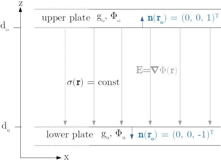
Mathematical formulation of the FEM Problem (for the interested and math affine reader only)
We start with our PDE in the so called strong form,
\begin{equation} -\nabla(\sigma \nabla \Phi) = 0 \end{equation}
which is then converted to the so called weak form. This is done by multiplying with a sufficiently smooth testfunction $v$, which additionally has to vanish on every point of the boundary where the solution to $\Phi$ is known and then integrating over the domain $\Omega$ \begin{equation} \int_{\Omega} -\nabla(\sigma \nabla \Phi) v \mathrm{dx} = 0. \end{equation} We then perform partial integration: $ \begin{equation} \int_{\Omega} \sigma (\nabla \Phi) \cdot (\nabla v) \mathrm{dx} - \int_{\partial \Omega} v \sigma (\nabla \Phi) \cdot \vec n \mathrm{ds} = 0 \end{equation} $ using Gauss’s theorem. The contribution of the so-called Dirichlet boundary conditions (BC), where the value of $\Phi$ on the part of the boundary is known, vanishes because $v$ vanishes on these parts of the boundary by definition of $v$ (see, e.g., Section 2.1.1 Langtangen16). The remaining boundaries are indexed by $i$ for so-called Robin-BC and $j$ for so-called Neumann-BC. Note that surface integrals coming from our Neumann boundary conditions also vanish \begin{equation} \int_{\Omega} \sigma (\nabla \Phi) \cdot (\nabla v) \mathrm{dx} - \sum_i \int_{\partial \Omega_{i, \mathrm{Robin}}} v g_i (\Phi_i - \Phi) \mathrm{dS} - \sum_j \int_{\partial \Omega_{j, \mathrm{Neumann}}} v g_j \mathrm{dS} = 0 \end{equation} because all $g_j = 0$.
We now rewrite the above equality by defining the so called bilinear $a(\Phi,v)$ and linear $L(v)$ term
\[a(\Phi,v) = \int_{\Omega} \sigma (\nabla \Phi) \cdot (\nabla v) \mathrm{dx} + \sum_i \int_{\partial \Omega_{i, \mathrm{Robin}}} v g_i \Phi \mathrm{dS}\] \[L(v) = \sum_i \int_{\partial \Omega_{i, \mathrm{Robin}}} v g_i \Phi_i \mathrm{dS} + \sum_j \int_{\partial \Omega_{j, \mathrm{Neumann}}} v g_j \mathrm{dS}.\]We now have to find a $\Phi$ element of the trial space $V$ and $v$ element of the test space $\hat V$ such that \begin{equation} a(\Phi,v) = L(v). \end{equation} Here $V$ and $\hat V$ are infinite-dimensional function spaces that guarantee that the above problem is well-defined (contains sufficiently smooth, well-behaved functions).
Because the Computer has a hard time working with infinite dimensional spaces we have to reduce to a finite dimensional space by putting the problem on a discrete mesh. Between each two nodes of the mesh the electrostatic potential is approximated as linear combination of finitely many polynomial basis functions. So we reduce to problem to find $\Phi \in V_{\mathrm h} \subset V$ and $v \in \hat V_{\mathrm h} \subset \hat V$, with $V_{\mathrm h}$ and $\hat V_{\mathrm h}$ finite dimensional such hat \begin{equation}a(\Phi,v) = L(v) \end{equation} (For more information see e.g. chapter 2.1 Langtangen16).
(A nice video illustrating how the FEM works in Detail for a simple 1 dimensional problem can be found here.)
references for learning how to write your own program
One of the things I love most about this project is that every part of the project is done by free to use open source software.
As mentioned before, you do not necessarily have to use (GMSH to create your geometry, there are other programs that do the same. Maybe you have obtained your geometry from measured data (e.g. MRI scan) and want to perform simulations with this geometry.)
The actual PDE is solved by fenics. I can’t recommend this software enough. It has an easy to use Python interface and is very robust and powerful. It has a large and very active community, so it’s easy to learn from others and improve. And what I like most is that the input to solve is very close to the actual mathematical formalism, so you understand more of what is going on. My recommodations for learning fenics are:
- fenics tutorial book This helps a lot if one wants to dig a bit deeper into the math and learn from examples how to use fenics. Be aware that some things are a bit outdated and you have to google as always if your get unexpected error messages. The community is big so there already was someone having the same problem.
- another fenics tutorial This is another nice tutorial to learn how to use fencis.
- the best tutorial for more realistic scenarios This blog is amazing. Here I learned how create easy geometries using CAD software, mesh them and use this as input for the fenics calculations.
For visualization, I recommend Paraview. However, if you have a very specific problem, you might think about using the output of the computation and writing your own visualization tools, e.g. with matplotlib.